Data Preprocessing

Data Preprocessing

1 . Data Cleaning.

Data cleaning routines attempt to fill in missing values, smooth out noise while identifying outliers, and correct inconsistencies in the data.

(i). Missing values

1. Ignore the tuple: This is usually done when the class label is missing (assuming the mining task involves classification or description). This method is not very effective, unless the tuple contains several attributes with missing values. It is especially poor when the percentage of missing values per attribute varies considerably.

2. Fill in the missing value manua

lly: In general, this approach is time-consuming and may not be feasible given a large data set with many missing values.

3. Use a global constant to fill in the missing value: Replace all missing attribute values by the same constant, such as a label like ―Unknown". If missing values are replaced by, say, ―Unknown", then the mining program may mistakenly think that they form an interesting concept, since they all have a value in common - that of ―Unknown". Hence, although this method is simple, it is not recommended.

4. Use the attribute mean to fill in the missing value: For example, suppose that the average income of All Electronics customers is $28,000. Use this value to replace the missing value for income.

5. Use the attribute mean for all samples belonging to the same class as the given tuple: For example, if classifying customers according to credit risk, replace the missing value with the average income value for customers in the same credit risk category as that of the given tuple.

6. Use the most probable value to fill in the missing value: This may be determined with inference-based tools using a Bayesian formalism or decision tree induction. For example, using the other customer attributes in your data set, you may construct a decision tree to predict the missing values for income.

(ii). Noisy data

Noise is a random error or variance in a measured variable.

1. Binning methods:

Binning methods smooth a sorted data value by consulting the ‖neighborhood", or values around it. The sorted values are distributed into a number of 'buckets', or bins. Because binning methods consult the neighborhood of values, they perform local smoothing. Figure illustrates some binning techniques.

In this example, the data for price are first sorted and partitioned into equi-depth bins (of depth 3). In smoothing by bin means, each value in a bin is replaced by the mean value of the bin. For example, the mean of the values 4, 8, and 15 in Bin 1 is 9. Therefore, each original value in this bin is replaced by the value 9. Similarly, smoothing by bin medians can be employed, in which each bin value is replaced by the bin median. In smoothing by bin boundaries, the minimum and maximum values in a given bin are identified as the bin boundaries. Each bin value is then replaced by the closest boundary value.

(i).Sorted data for price (in dollars): 4, 8, 15, 21, 21, 24, 25, 28, 34 (ii).Partition into (equi-width) bins:

Bin 1: 4, 8, 15

Bin 2: 21, 21, 24

Bin 3: 25, 28, 34

(iii).Smoothing by bin means:

Bin 1: 9, 9, 9,

Bin 2: 22, 22, 22

Bin 3: 29, 29, 29

(iv).Smoothing by bin boundaries:

Bin 1: 4, 4, 15

Bin 2: 21, 21, 24

Bin 3: 25, 25, 34

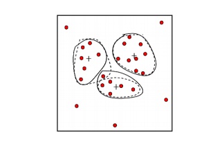
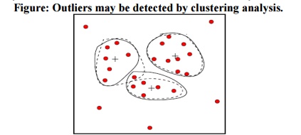
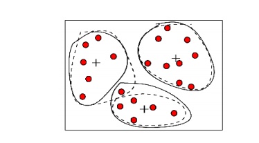
2. Clustering:

Outliers may be detected by clustering, where similar values are organized into groups or

―clusters‖. Intuitively, values which fall outside of the set of clusters may be considered outliers.

Figure: Outliers may be detected by clustering analysis.

3. Combined computer and human inspection: Outliers may be identified through a combination of computer and human inspection. In one application, for example, an information-theoretic measure was used to help identify outlier patterns in a handwritten character database for classification. The measure's value reflected the ―surprise" content of the predicted character label with respect to the known label. Outlier patterns may be informative or ―garbage". Patterns whose surprise content is above a threshold are output to a list. A human can then sort through the patterns in the list to identify the actual garbage ones

4. Regression: Data can be smoothed by fitting the data to a function, such as with regression.

Linear regression involves finding the ―best" line to fit two variables, so that one variable can be used to predict the other. Multiple linear regression is an extension of linear regression, where more than two variables are involved and the data are fit to a multidimensional surface.

(iii). Inconsistent data

There may be inconsistencies in the data recorded for some transactions. Some data inconsistencies may be corrected manually using external references. For example, errors made at data entry may be corrected by performing a paper trace. This may be coupled with routines designed to help correct the inconsistent use of codes. Knowledge engineering tools may also be used to detect the violation of known data constraints. For example, known functional dependencies between attributes can be used to find values contradicting the functional constraints.

2. Data Transformation.

In data transformation, the data are transformed or consolidated into forms appropriate for mining. Data transformation can involve the following:

Normalization, where the attribute data are scaled so as to fall within a small specified range, such as -1.0 to 1.0, or 0 to 1.0.

There are three main methods for data normalization : min-max normalization, z-score

normalization, and normalization by decimal scaling.

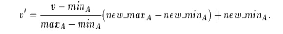
(i).Min-max normalization performs a linear transformation on the original data. Suppose that minA and maxA are the minimum and maximum values of an attribute A. Min-max normalization maps a value v of A to v0 in the range [new minA; new maxA] by computing

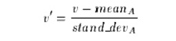
(ii).z-score normalization (or zero-mean normalization), the values for an attribute A are normalized based on the mean and standard deviation of A. A value v of A is normalized to v0 by computing where mean A and stand dev A are the mean and standard deviation, respectively, of attribute A. This method of normalization is useful when the actual minimum and maximum of attribute A are unknown, or when there are outliers which dominate the min-max normalization.

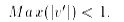
(iii). Normalization by decimal scaling normalizes by moving the decimal point of values of attribute A. The number of decimal points moved depends on the maximum absolute value of A. A value v of A is normalized to v0by computing where j is the smallest integer such that

Smoothing, which works to remove the noise from data? Such techniques include binning, clustering, and regression.

(i). Binning methods:

Binning methods smooth a sorted data value by consulting the ‖neighborhood", or values around it. The sorted values are distributed into a number of 'buckets', or bins. Because binning methods consult the neighborhood of values, they perform local smoothing. Figure illustrates some binning techniques.

In this example, the data for price are first sorted and partitioned into equi-depth bins (of depth 3). In smoothing by bin means, each value in a bin is replaced by the mean value of the bin. For example, the mean of the values 4, 8, and 15 in Bin 1 is 9. Therefore, each original value in this bin is replaced by the value 9. Similarly, smoothing by bin medians can be employed, in which each bin value is replaced by the bin median. In smoothing by bin boundaries, the minimum and maximum values in a given bin are identified as the bin boundaries. Each bin value is then replaced by the closest boundary value.

(i).Sorted data for price (in dollars): 4, 8, 15, 21, 21, 24, 25, 28, 34 (ii).Partition into (equi-width) bins:

Bin 1: 4, 8, 15

Bin 2: 21, 21, 24

Bin 3: 25, 28, 34

(iii).Smoothing by bin means:

Bin 1: 9, 9, 9,

Bin 2: 22, 22, 22

Bin 3: 29, 29, 29

(iv).Smoothing by bin boundaries:

Bin 1: 4, 4, 15

Bin 2: 21, 21, 24

Bin 3: 25, 25, 34

(ii). Clustering:

Outliers may be detected by clustering, where similar values are organized into groups or

―clusters‖. Intuitively, values which fall outside of the set of clusters may be considered outliers.

Figure: Outliers may be detected by clustering analysis.

Aggregation, where summary or aggregation operations are applied to the data. For example, the daily sales data may be aggregated so as to compute monthly and annual total amounts.

Generalization of the data, where low level or 'primitive' (raw) data are replaced by higher level concepts through the use of concept hierarchies. For example, categorical attributes, like street, can be generalized to higher level concepts, like city or county.

3. Data reduction.

Data reduction techniques can be applied to obtain a reduced representation of the data set that is much smaller in volume, yet closely maintains the integrity of the original data. That is, mining on the reduced data set should be more efficient yet produce the same (or almost the same) analytical results.

Strategies for data reduction include the following.

Data cube aggregation, where aggregation operations are applied to the data in the construction of a data cube.

Dimension reduction, where irrelevant, weakly relevant or redundant attributes or dimensions may be detected and removed.

Data compression, where encoding mechanisms are used to reduce the data set size.

Numerosity reduction, where the data are replaced or estimated by alternative, smaller data representations such as parametric models (which need store only the model parameters instead of the actual data), or nonparametric methods such as clustering, sampling, and the use of histograms.

Discretization and concept hierarchy generation, where raw data values for attributes are replaced by ranges or higher conceptual levels. Concept hierarchies allow the mining of data at multiple levels of abstraction, and are a powerful tool for data mining.

Data Cube Aggregation

The lowest level of a data cube

the aggregated data for an individual entity of interest

e.g., a customer in a phone calling data warehouse.

Multiple levels of aggregation in data cubes

Further reduce the size of data to deal with

Reference appropriate levels

Use the smallest representation which is enough to solve the task

Queries regarding aggregated information should be answered using data cube, when possible

Dimensionality Reduction

Feature selection (i.e., attribute subset selection):

Select a minimum set of features such that the probability distribution of different classes given the values for those features is as close as possible to the original distribution given the values of all features

reduce # of patterns in the patterns, easier to understand

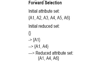
Heuristic methods:

Step-wise forward selection: The procedure starts with an empty set of attributes. The best of the original attributes is determined and added to the set. At each subsequent iteration or step, the best of the remaining original attributes is added to the set.

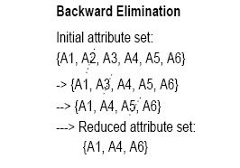
Step-wise backward elimination: The procedure starts with the full set of attributes. At each step, it removes the worst attribute remaining in the set.

Combination forward selection and backward elimination: The step-wise forward selection and backward elimination methods can be combined, where at each step one selects the best attribute and removes the

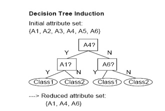
Decision tree induction: Decision tree algorithms, such as ID3 and C4.5, were originally intended for classifcation. Decision tree induction constructs a flow-chart-like structure where each internal (non-leaf) node denotes a test on an attribute, each branch corresponds to an outcome of the test, and each external (leaf) node denotes a class prediction. At each node, the algorithm chooses the ―best" attribute to partition the data into individual classes.

Data compression

In data compression, data encoding or transformations are applied so as to obtain a reduced or ‖compressed" representation of the original data. If the original data can be reconstructed from the compressed data without any loss of information, the data compression technique used is called lossless. If, instead, we can reconstruct only an approximation of the original data, then the data compression technique is called lossy. The two popular and effective methods of lossy data compression: wavelet transforms, and principal components analysis.

Wavelet transforms

The discrete wavelet transform (DWT) is a linear signal processing technique that, when applied to a data vector D, transforms it to a numerically different vector, D0, of wavelet coefficients. The two vectors are of the same length.

The DWT is closely related to the discrete Fourier transform (DFT), a signal processing technique involving sines and cosines. In general, however, the DWT achieves better lossy compression.

The general algorithm for a discrete wavelet transform is as follows.

The length, L, of the input data vector must be an integer power of two. This condition can be met by padding the data vector with zeros, as necessary.

Each transform involves applying two functions. The first applies some data smoothing, such as a sum or weighted average. The second performs a weighted difference.

The two functions are applied to pairs of the input data, resulting in two sets of data of length L=2. In general, these respectively represent a smoothed version of the input data, and the high-frequency content of it.

The two functions are recursively applied to the sets of data obtained in the previous loop, until the resulting data sets obtained are of desired length.

A selection of values from the data sets obtained in the above iterations are designated the wavelet coefficients of the transformed data.

Principal components analysis

Principal components analysis (PCA) searches for c k-dimensional orthogonal vectors that can best be used to represent the data, where c << N. The original data is thus projected onto a much smaller space, resulting in data compression. PCA can be used as a form of dimensionality reduction. The initial data can then be projected onto this smaller set.

The basic procedure is as follows.

The input data are normalized, so that each attribute falls within the same range. This step helps ensure that attributes with large domains will not dominate attributes with smaller domains.

PCA computes N orthonormal vectors which provide a basis for the normalized input data. These are unit vectors that each point in a direction perpendicular to the others. These vectors are referred to as the principal components. The input data are a linear combination of the principal components.

The principal components are sorted in order of decreasing ―significance" or strength. The principal components essentially serve as a new set of axes for the data, providing important information about variance.

since the components are sorted according to decreasing order of ―significance", the size of the data can be reduced by eliminating the weaker components, i.e., those with low variance. Using the strongest principal components, it should be possible to reconstruct a good approximation of the original data.

Numerosity reduction Regression and log-linear models

Regression and log-linear models can be used to approximate the given data. In linear regression, the data are modeled to fit a straight line. For example, a random variable, Y (called a response variable), can be modeled as a linear function of another random variable, X (called a predictor variable), with the equation where the variance of Y is assumed to be constant. These coefficients can be solved for by the method of least squares, which minimizes the error between the actual line separating the data and the estimate of the line.

Multiple regression is an extension of linear regression allowing a response variable Y to be modeled as a linear function of a multidimensional feature vector.

Log-linear models approximate discrete multidimensional probability distributions. The method can be used to estimate the probability of each cell in a base cuboid for a set of discretized attributes, based on the smaller cuboids making up the data cube lattice

Histograms

A histogram for an attribute A partitions the data distribution of A into disjoint subsets, or buckets. The buckets are displayed on a horizontal axis, while the height (and area) of a bucket typically reects the average frequency of the values represented by the bucket.

Equi-width: In an equi-width histogram, the width of each bucket range is constant (such as the width of $10 for the buckets in Figure 3.8).

Equi-depth (or equi-height): In an equi-depth histogram, the buckets are created so that, roughly, the frequency of each bucket is constant (that is, each bucket contains roughly the same number of contiguous data samples).

V-Optimal: If we consider all of the possible histograms for a given number of buckets, the V-optimal histogram is the one with the least variance. Histogram variance is a weighted sum of the original values that each bucket represents, where bucket weight is equal to the number of values in the bucket.

MaxDiff: In a MaxDiff histogram, we consider the difference between each pair of adjacent values. A bucket boundary is established between each pair for pairs having the Beta largest differences, where Beta-1 is user-specified.

Clustering

Clustering techniques consider data tuples as objects. They partition the objects into groups or clusters, so that objects within a cluster are ―similar" to one another and ―dissimilar" to objects in other clusters. Similarity is commonly defined in terms of how ―close" the objects are in space, based on a distance function. The ―quality" of a cluster may be represented by its diameter, the maximum distance between any two objects in the cluster. Centroid distance is an alternative measure of cluster quality, and is defined as the average distance of each cluster object from the cluster centroid.

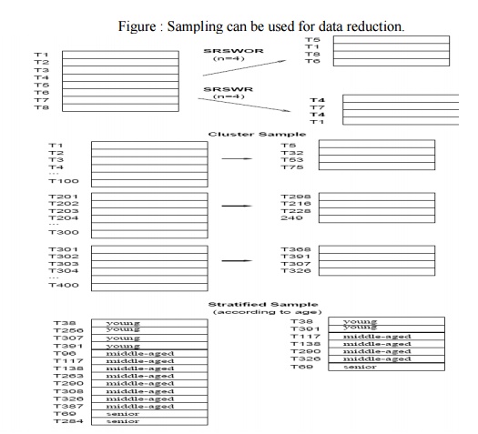
Sampling

Sampling can be used as a data reduction technique since it allows a large data set to be represented by a much smaller random sample (or subset) of the data. Suppose that a large data set, D, contains N tuples. Let's have a look at some possible samples for D.

Simple random sample without replacement (SRSWOR) of size n: This is created by drawing n of the N tuples from D (n < N), where the probably of drawing any tuple in D is 1=N, i.e., all tuples are equally likely.

Simple random sample with replacement (SRSWR) of size n: This is similar to SRSWOR, except that each time a tuple is drawn from D, it is recorded and then replaced. That is, after a tuple is drawn, it is placed back in D so that it may be drawn again.

Cluster sample: If the tuples in D are grouped into M mutually disjoint ―clusters", then a SRS of m clusters can be obtained, where m < M. A reduced data representation can be obtained by applying, say, SRSWOR to the pages, resulting in a cluster sample of the tuples.

Stratified sample: If D is divided into mutually disjoint parts called ―strata", a stratified sample of D is generated by obtaining a SRS at each stratum. This helps to ensure a representative sample, especially when the data are skewed. For example, a stratified sample may be obtained from customer data, where stratum is created for each customer age group.